APPENDIX B
DETAILS OF THE TOPOGRAPHIC TEMPERATURE MODELS
The two methods of determining the thermal emission from a macroscopically
rough surface, used in Chapter 6, are here discussed in detail.
Model A: Adaption of the Results of
Winter and Krupp (1971)
Winter and Krupp (1971) were considering the observed beaming of 11\dmic\
thermal emission from individual regions on the Earth's Moon (see
Appendix A). Their model calculated temperatures across an idealized
rough surface (a plane indented with spherical-section craters) and successfully
explained the beaming as due to these topographic temperature variations.
They calculated the temperature at each point in an obliquely-illuminated
crater of albedo A = 0.08, by considering the direct solar insolation
(if any) at that point, and the thermal radiation absorbed from the rest
of the crater interior. They also allowed for radial sub-surface conduction
of heat but concluded that, using lunar surface thermal inertias, conduction
did not affect crater temperatures very much. They did not include scattered
sunlight within the crater, which may be a reasonable assumption given
the low albedo of the Moon.
Note that in this appendix, A is a `single-scattering' albedo.
As photons in the model can encounter the rough surface more than once
and thus have more than one chance to be absorbed, the actual surface albedo
will be lower than A by an amount that will depend on the geometry
of the surface and the lighting conditions.
Figures 6 and 7 of Winter and Krupp (1971) show calculated temperature
profiles along the meridian (the line of symmetry aligned with the direction
of the sun) of spherical-section `craters'. Profiles are given for a hemispherical
crater (depth/diameter ratio, D, = 0.5) at solar incidence angles
of 0o, 30o, 60o, 70o, and 80o,
and a more subdued crater (D = 0.25) at 0o, 30o,
and 60o. I digitized these profiles, and scaled them to Callisto
surface temperatures by multiplying by the ratio of the subsolar temperature
observed by Voyager on Callisto (158oK) to the lunar subsolar
temperature used by Winter and Krupp (385.5oK).
The temperature information provided by Winter and Krupp pertains only
to the crater meridian: they do not give temperatures elsewhere in the
crater so a calculation of the thermal emission from the crater in three
dimensions is not possible. I therefore used the temperature profile in
a two-dimensional calculation, applying it to an infinite trench with the
same circular-arc profile as the crater cross-section. This introduces
an error: the geometry of the trench is different and the actual temperature
profile within it will be somewhat different from that within a three-dimensional
crater. However, this simplification allows the calculation of results
that should be at least qualitatively valid. Figure
42 illustrates the model.
Calculation of Thermal Emission
The results of the IRIS spectrum fitting (Chapter 4) indicate a wavelength-independent
emissivity typically about 0.94, rather than unity, for the surfaces of
the Galilean satellites. This is not included in the Winter and Krupp model,
which assumes unit emissivity, but has a significant effect on the shape
of the final spectrum. Therefore a non-unit emissivity \ep\ is simulated
by increasing the temperature of each point on the crater profile by the
factor \ep-0.25 (this is the effect of non-unit emissivity on
the equilibrium temperature of a smooth surface):

The radiated flux from each surface element is then reduced by the
factor \ep\ at all wavelengths in Equation 18 below.
Simple (but tedious) geometry determines what portions of the trench
interior are visible from a given emission angle. The visible opening of
the trench is divided into ten sections of equal projected area and the
location of the center of each within the crater is determined. The temperature
at that point is read from the digitized and scaled temperature profile,
interpolating as necessary. This gives ten temperatures Tj,
all contributing equally to the thermal emission viewed from this angle.
The thermal emission spectrum $R(\lambda)$ of a surface with fractional
trench coverage X and emissivity \ep\ is given by the weighted combination
of blackbody spectra at the temperatures of each of the visible surface
elements:

where xj, the fraction of the projected trench area,
seen at a given emission angle, that is occupied by element j, is
always 0.1 in this case. $B(\lambda,T)$ is the Planck function at wavelength
$\lambda$ and temperature T. The temperature of a horizontal surface
outside the trench, Th, was also obtained from Winter
and Krupp (1971) Figs. 6 and 7, and scaled in the same way as the interior
temperatures.
The spectrum $R(\lambda)$ can be compared directly with the IRIS spectra,
or can be fitted with a 2-component blackbody in an identical way to the
IRIS spectra so that the fit parameters can be compared.
I ran this model for all combinations of the following values of the
input parameters: both available values of D (0.5 and 0.25), all
solar incidence angles available for each D (0o, 30o,
60o, 70o, 80o for D = 0.5 and 0o,
30o, 60o for D = 0.25), X = 0.1 and
0.6, and emission angle = 0o, and 30o and 60o
on
each side of the vertical. \ep\ was held at 0.94. The results are in Fig.
21, in Chapter 6 of the main body of the text. Emission angles of 60o
often gave spectrum shapes very different from smaller values and were
not plotted in order to keep the ribbons narrow enough to be useful. The
great majority of the plotted IRIS spectra have emission angles less than
60o, anyway.
Model B: Triangular Trench
Whereas Winter and Krupp (1971) and Hansen (1977) considered spherical-surfaced
craters, the model I have constructed is only two dimensional, and considers
the temperature distribution within an infinite trench. It is otherwise
similar to the abovementioned models, though unlike them it includes scattered
solar radiation and is thus valid for high albedo surfaces. Emissivity
is assumed to be unity, in order to avoid the complex calculation of scattered
thermal radiation. A non-unit emissivity can, however, be simulated in
calculating the final thermal emission spectrum.
Trench Geometry
The trench has an icoseles triangle cross-section, with vertical walls
and a depth/half-width ratio of D. See Fig.
43 for an illustration. Three surface elements are considered: the
wall facing away from the sun (1), and the shadowed (2) and illuminated
(3) portions of the sun-facing wall. The area of element 2 is zero if the
sun is high enough to illuminate the bottom of the trench.
The model first calculates the size of each surface element, a function
of D and the solar incidence angle i, and from this, by straightforward
geometry, the fractional solid angle (fraction of a full hemisphere)
fjk subtended by every element k as seen from the
center of each other element j.
Calculation of Scattered Light (Solar Radiation)
For a given surface element j, the flux Fj of
light scattered from it is related to the flux of incident scattered and
direct light by the `single-scattering' albedo A:
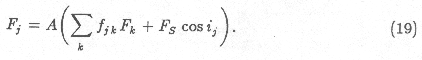
FS is the incident direct solar flux (zero if the
element is in shadow, i.e. for elements 2 and sometimes 1) and ij
is
the solar incidence angle relative to the local surface normal. Solution
of the three linear simultaneous equations for Fj is
accomplished by matrix inversion.
A major (and invalid) assumption implicit in Equation 19 is that conditions
are the same over the whole of each surface element, i.e.\ the flux Fj
and
the projection factor fjk applies over the whole of element
j.
A more thorough model would subdivide each surface element for greater
accuracy, but the assumption of constancy over each element (also assumed
in the following calculation of temperatures) should give useful first-order
results.
Calculation of Temperatures
Calculation of the temperature Tj of each surface element
is similar to the calculation of scattered light. Zero thermal inertia
is assumed, so that the temperature is that for which emitted thermal radiation
balances absorbed incident radiation (direct and scattered solar, and thermal
radiation from other surface elements):
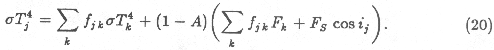
All Fk's have already been determined, so this gives
three simultaneous linear equations in Tj4,
which are again solved by matrix inversion. Equation 20 assumes unit emissivity
so that scattered thermal radiation can be ignored.
Finally, the temperature Th of a horizontal surface
outside the trench is given simply by
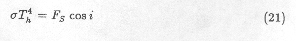
where i is the solar incidence angle.
Calculation of Thermal Emission
Non-unit emissivity, needed to produce emission spectra comparable to those
of the Galilean satellites, is simulated as in model A, by increasing the
temperature of each surface element by the factor \ep-0.25,
and then reducing the radiated flux by \ep\ in Equation 18.
Finally, the thermal emission spectrum from the trench and its surroundings
is calculated using Equation 18 as in model A. xj, the
fraction of the projected trench area, seen at a given emission angle,
that is occupied by element j, is not constant this time, but can
be calculated by simple geometry.
The resulting spectrum is treated as in model A, being compared directly
with the IRIS spectra or first fitted with a 2-component blackbody.
I ran model B with the same range of parameters as model A, with the
additional variable A (albedo) given values of 0.2 and 0.45. Also,
unlike model A, I was able to use solar incidence angles of 70o
and 80o with D=0.25. The results are in
Figs. 19 and 20, in Chapter 6 of the main
body of the text. As with model A, and for the same reasons, emission angles
of 60o were not plotted.